Phonon calculations with small displacement method

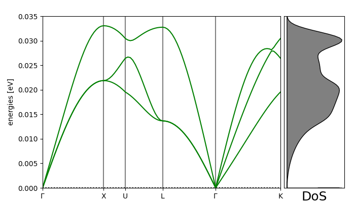
Simple example showing how to calculate the phonon dispersion for bulk aluminum using a 5x5x5 supercell within effective medium theory:

import matplotlib.pyplot as plt
import numpy as np

from ase.build import bulk
from ase.calculators.emt import EMT
from ase.phonons import Phonons

Setup Al crystal

atoms = bulk('Al', 'fcc', a=4.05)

Setup phonon calculation with EMT calculator

N = 5
ph = Phonons(
    atoms,
    EMT(),
    supercell=(N, N, N),
    use_mean_minimum_images=True,
    minimum_image_tol=1e-6,
)
ph.run()

Read forces and assemble the dynamical matrix

ph.read()
ph.clean()

7

Set and plot phonon band-structure along specific path

path = atoms.cell.bandpath('GXULGK', npoints=100)
bs = ph.get_band_structure(path)

# Get phonon DoS
dos = ph.get_dos(kpts=(20, 20, 20)).sample_grid(npts=100, width=1e-3)
fig = plt.figure(figsize=(7, 4))
ax = fig.add_axes([0.12, 0.07, 0.67, 0.85])

# Plot phonon band structure and DoS
emax = 0.035
bs.plot(ax=ax, emin=0.0, emax=emax)

dosax = fig.add_axes([0.8, 0.07, 0.17, 0.85])
dosax.fill_between(
    dos.get_weights(),
    dos.get_energies(),
    y2=0,
    color='grey',
    edgecolor='k',
    lw=1,
)

dosax.set_ylim(0, emax)
dosax.set_yticks([])
dosax.set_xticks([])
dosax.set_xlabel('DoS', fontsize=18)
plt.show()

# fig.savefig('Al_phonon.png')

WARNING, 1 imaginary frequencies at q = ( 0.00,  0.00,  0.00) ; (omega_q = 5.742e-09*i)
WARNING, 1 imaginary frequencies at q = ( 0.00,  0.00,  0.00) ; (omega_q = 5.742e-09*i)

You can visualize the modes with the following script:

# Write modes for specific q-vector to trajectory file
L = np.array(path.special_points['L'])
ph.write_modes(
    L / 2.0,
    branches=[2],
    repeat=(8, 8, 8),
    kT=3e-4,
    center=True,
)

# Optionally, generate gif animation

# from ase.io.trajectory import Trajectory
# from ase.io import write

# Temporarily disabled due to matplotlib writer compatibility issue.
# with Trajectory('phonon.mode.2.traj', 'r') as traj:
#    write('Al_mode.gif', traj, interval=50,
#           rotation='-36x,26.5y,-25z')